Have you ever wished to show off your artistic talent by turning your images into a sketch or painting? You can achieve that using several built-in OpenCV methods! A strong library for computer vision and image processing is OpenCV. You will learn how to use OpenCV in Python to convert your photographs into sketches and paints in this project.

1)Import Libraries and Load your Images

import numpy as np 
import matplotlib.pyplot as plt
import cv2

The OpenCV library, cv2, matplotlib. pyplot, which will be used to plot our photos, and the numpy library for matrices computations.

img = cv2.imread("./images/Monolisa.jpeg") 
plt.imshow(img)

We will use the cv2.imread() method to load the image file. The path to an image is the input parameter for this method, which reads an image into a numpy array. Based on the number of color channels contained in the image, the algorithm returns a matrix.

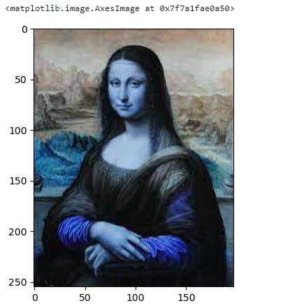
You might have noticed that the colors didn't seem quite right. This is because while OpenCV reads the image's color channels in a BGR order, the original image's color channels might have been RGB.

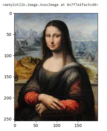
We can fix this by using the cv2.cvtColor() method with the input parameters of the picture and cv2.COLOR BGR2RGB to signal that we are converting the image from the form BGR to RGB.

img_rgb = cv2.cvtColor(img, cv2.COLOR_BGR2RGB)
plt.imshow(img_rgb)

Note: Images are either grayscale or colored. A pixel defines a point in an image. Unlike us humans, when a computer sees an image, it doesn't see shapes and colors but rather a matrix of numbers. Colored images usually have 3 color channels and are of the form BGR (Blue-Green-Red) or RGB (Red-Green-Blue). Grayscale images only have one color channel and every pixel value is a number between 0 and 255. 0 indicates the color black and 255 indicates white.

2)Convert Your Picture To Grayscale

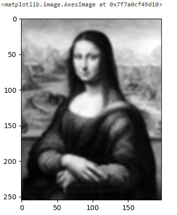
As grayscale photos only have one color channel but colored images have three, it is frequently necessary to transform colorful images to grayscale in the preprocessing stage to speed up calculation. Moreover, color information typically doesn't assist us in locating the features we seek. The cv2.cvtColor() method in OpenCV can change a colored image into a grayscale one. The image you wish to convert is indicated by the first parameter, img, and the second parameter, cv2. COLOR BGR2GRAY, denotes that you want to convert your image from a BGR image to a grayscale image.

gray = cv2.cvtColor(img, cv2.COLOR_BGR2GRAY)
plt.imshow(gray, cmap = 'gray')

3)Smooth Your Picture

To lessen an image's noise, a smoothing filter is frequently applied. Random fluctuations in brightness are known as picture noise. Typically, it can be seen in your photo's grainy areas. Your image becomes more blurry as a result of image smoothing. The Gaussian filter is a widely used smoothing filter.

The cv2.GaussianBlur() method in OpenCV blurs a picture using the Gaussian filter. The method requires three parameters: the image you want to smooth, the size of the filter (for example, a parameter value of (5,5) suggests a square filter with sides that are each 5 pixels long), and the sigma value. The sigma parameter determines how fuzzy your image will be.

blur = cv2.GaussianBlur(gray,(5,5),2)
plt.imshow(blur, cmap = 'gray')

Now try for Higher sigma Values

smoothed= cv2.GaussianBlur(gray,(7,7),5)                   
plt.imshow(smoothed)

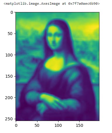
You'll observe that the resultant image grows increasingly hazy as sigma increases. You might think of it like this: the more information you want to remove from the image, the greater must be the sigma value. So, you must select a suitable sigma value such that key image elements are preserved when the Gaussian filter is applied.

4) Edge Detection

The areas of an image where brightness fluctuates quickly are its edges. We must calculate something called the gradient magnitude of a picture to find the image's edges. A picture's gradient magnitude, which is employed for edge identification, quantifies how quickly the image is changing. We will calculate the image's gradient magnitude to obtain a sketch for our snapshot.

We apply a filter known as the Sobel filter to the photos to calculate how much the image changes in each direction. We employ the method cv2. Sobel() in OpenCV to accomplish this.

sobelx = cv2.Sobel(blur,cv2.CV_64F,1,0,ksize=5) # Change in horizonal direction, dx
sobely = cv2.Sobel(blur,cv2.CV_64F,0,1,ksize=5) # Change in verticle direction, dy
gradmag_sq = np.square(sobelx)+np.square(sobely) # Square the images element-wise and then add them together 
gradmag = np.sqrt(gradmag_sq) # Take the square root of the resulting image element-wise to get the gradient magnitude

plt.imshow(gradmag, cmap ='gray')

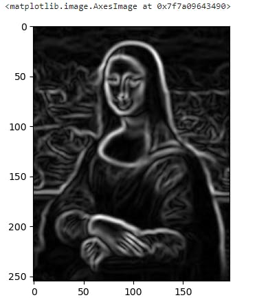
We will now reverse the colors of the gradient magnitude of the image.

gradmag_inv = 255-gradmag 
plt.imshow(gradmag_inv, cmap = "gray")

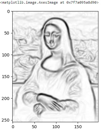
You can use the threshold of your image to create a sketch of your shot with only black and white as the colors. The cv2.threshold method in OpenCV can be used to determine an image's threshold (). This method returns a tuple, where the threshold value is the first element and the thresholded image is the second. There are other types of thresholding where the threshold value needs to be computed, but for the thresholding method we will be using in this task, we will be providing the threshold value in the input.

thresh_value, thresh_img = cv2.threshold(gradmag_inv,10,255,cv2.THRESH_BINARY)
plt.imshow(thresh_img, cmap = 'gray')

The parameters of this method are src, three, maximal and type. src is a grayscale image, this is your threshold value, maxval is the maximum value you are assigning to a pixel and type is the type of thresholding you want to use. As you will see in the code cell below, the threshold value we have set is 10, the maximum value is 255 and the thresholding method we have set is cv2.THRESH_BINARY. cv2.THRESH_BINARY just indicates that if the pixel value is less than the threshold value then set the value to 0, otherwise set the value to 255.

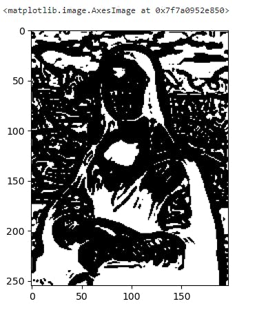
Thresholding is a technique for converting a grayscale (pixel values between 0 and 255) image into a binary image. A binary image is one in which each pixel can have one of two values, often 0 (black) or 255. (white). The way the method commonly operates is that for a threshold value between 0 and 255 if the pixel value is less than that value, it is mapped to 0 (black), and if it is larger than that value, it is mapped to the maximum value, typically 255. (white).

5)Pencil Sketch

To create a pencil sketch from your photo, use OpenCV's cv2.pencilSketch() function.

A grayscale and colored pencil sketch of the input image is both returned by the function cv2.pencilSketch(). Our original colored image from Exercise 1, img RGB, in which the colors appeared as they should, will be our input image. As you can see from the code below, the method also accepts the arguments sigma s, sigma r, and shade factor.

How smooth you want the final image to be can be set using the sigma s parameter, which has a range of 0-200. The smoother the image, the greater the value of sigma s.

How much you want distinct colors in your image to blend is determined by sigma r, a value between 0 and 1. If your sigma r-value is low, you should only consider related regions. This value is crucial if you want to keep an image's edges when you smooth it.

The shade factor ranges from 0.0 to 1.0. The brightness of the image increases with the shade factor's value.

pencilsketch_gray, pencilsketch_color  = cv2.pencilSketch(img_rgb, sigma_s=60, sigma_r=0.07, shade_factor=0.05) 

plt.imshow(pencilsketch_gray, cmap ='gray')

Actually, code derived image is not so well try using different parameters